Re-Identification Risk vs k-Anonymity: An Experimental Walkthrough
Most discussions of anonymization focus on buzzwords like k-anonymity and differential privacy, but few dig into what actually happens to a dataset as anonymity strength increases.
In this post, we conduct a full experimental walkthrough to quantify how raising the k-anonymity level impacts both privacy (re-identification risk) and data utility.
We simulate an attacker with partial knowledge trying to re-identify individuals, and we measure how data quality degrades as we ramp up the anonymization.
The goal is to illuminate where the balance lies between keeping data useful and keeping individuals anonymous.
Data Generation and Anonymization Setup
For our experiment, we generated a synthetic dataset of 2,000 individuals, each with the following fields:
| Field | Description |
|---|---|
age |
Numerical age (used as a quasi-identifier) |
zip3 |
3-digit ZIP code prefix (regional location, quasi-identifier) |
sex |
Binary sex attribute (quasi-identifier) |
lab_glucose |
Continuous lab glucose level (a target variable not used in anonymization) |
We treat age, zip3, and sex as the quasi-identifiers (QIs) that will be subject to anonymization.
The value of k in k-anonymity was varied from 1 to 20.
A k-anonymity requirement means each record must be indistinguishable from at least k–1 others with respect to these QIs.
To achieve this, an anonymization routine groups and generalizes records until every combination of QIs occurs in at least k records.
In practical terms, as k increases, the algorithm must increasingly generalize (coarsen) or suppress details in the QIs to satisfy the larger group size.
Parameters explored
We explored a few key parameters that control how the data is generalized:
- Age bin width: We varied age grouping from 1-year bins (no grouping beyond integer ages) up to 10-year bins. Larger bin widths mean ages get lumped into broader ranges (e.g., 30–39).
- Top-coding of age: Extreme ages were top-coded above a threshold (e.g., all ages 75 and above recorded as
"75+"). This prevents very old ages from standing out. - Rare ZIP suppression: Low-frequency ZIP3 regions were grouped into an
"Other"category once their count fell below a threshold. If a region is too unique, it gets collapsed to hide outliers.
By adjusting these knobs, we impose different anonymization strategies.
For each value of k (and each combination of binning/top-coding settings), we produced an anonymized version of the dataset and evaluated how much information was lost in the process.
Attacker Context: Partial Knowledge Threat Model
Anonymization is only meaningful relative to an attacker’s knowledge.
In our scenario, we simulate an attacker who has partial information about individuals — specifically, the attacker knows an individual’s:
- age
- general location (ZIP3 region)
- sex
(e.g., from a data leak or public records).
This is a common threat model for re-identification:
an adversary might obtain someone’s demographic details from a breached source and then try to find that person in an anonymized dataset (such as medical or survey data) released publicly.
The attacker’s goal is re-identification:
to match each anonymized record to the corresponding real individual by comparing the quasi-identifiers.
Importantly, the attacker does not know the sensitive value (lab_glucose) in our case;
they only leverage the QIs that are also present (albeit generalized) in the anonymized data.
This kind of attack is known as a record linkage attack, using the assumption that if an anonymized entry shares a unique combination of age, region, and sex with a known individual’s data, they are likely the same person.
This threat model underscores why k-anonymity focuses on QIs:
even innocuous-seeming attributes like age and ZIP code can triangulate someone’s identity when combined.
Next, we describe how our simulated attacker performs the re-identification.
Attacker’s Re-identification Strategy (Global Matching)
How does our attacker try to re-identify records?
Instead of using a simple greedy matching (checking each anonymized record independently),
we implement a global optimization strategy.
We use a bipartite assignment solver (Google OR-Tools’ linear sum assignment solver) to find the optimal one-to-one matching between anonymized records and original records that best aligns their attributes.
Cost-based Matching
We define a cost for matching an anonymized record aᵢ with an original record oⱼ based on their differences in quasi-identifiers:
cost(i, j) = d_age(a_i, o_j) + d_zip(a_i, o_j) + d_sex(a_i, o_j)
Each d term is a distance measure for that attribute.
- If an anonymized age is a range (due to binning) and the original age falls within that range, the age distance may be zero; if it falls outside, the distance increases.
- If an anonymized ZIP3 was generalized to
"Other", any specific ZIP from the original will incur a cost when compared to"Other".
These distances capture how well an original record fits the generalized form of an anonymized record.
Lower cost → the two records are more similar across QIs.
We then solve for the assignment π(i) that minimizes the total cost of matching all anonymized records to distinct original records:
min_π  Σ_i  cost(i, π(i))
subject to: each original record is matched at most once
This optimization finds the best overall matching between the two datasets.
By considering all records jointly, the attacker avoids making locally optimal but globally inconsistent matches.
Even if each anonymized record individually has multiple plausible matches, the solver finds a globally consistent assignment.
The outcome is an assignment pairing most anonymized records with specific original record guesses.
Measuring Re-identification Success: Hit@1
To evaluate the attack, we use the Hit@k metric common in information retrieval.
A “hit” means the correct original record appears within the attacker’s top k guesses for an anonymized record.
In our case:
- the solver produces one best match per anonymized record
→ effectively Hit@1 only
So we focus on Hit@1, the fraction of anonymized records where the attacker’s top guess is correct.
A Hit@1 of 50% means the attacker correctly re-identified half of the individuals on the first guess.
(Hit@5 would allow up to 5 guesses per record, but we stick with the strictest measure.)
With the attack strategy and success metric defined, we now examine how re-identification risk and data utility change as anonymization strength increases.
Results
Re-identification Success vs. Anonymity Level
We first examine how the attacker’s success rate (Hit@1) changes as the anonymity parameter k increases.
Intuitively, higher k (stronger anonymity) should make re-identification harder.
Our experiments confirmed this:
the attacker’s success drops dramatically as k grows.
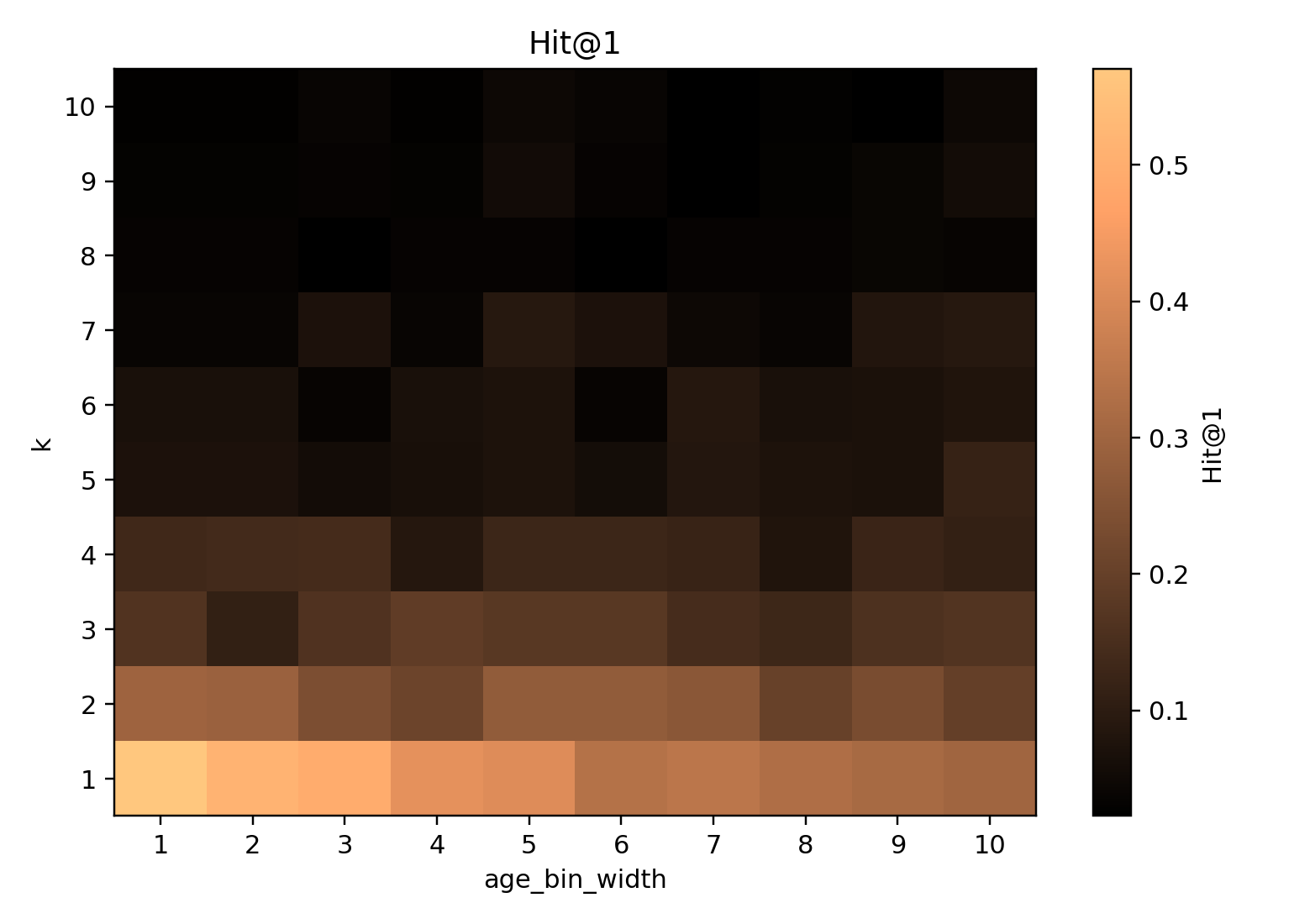
Each cell is the average Hit@1 across trials for a given combination of k (y-axis) and age bin width (x-axis). Success rates plummet as k increases. Notably, there is a sharp drop in attacker success once k is around 5–7, indicating the onset of strong anonymity where the attack loses traction.*
Even at k = 1 (minimal anonymization), the attacker does not get a 100% hit rate.
The maximum Hit@1 observed hovered just above ~50%.
This is because even in the raw data, some individuals share the same QI values
(e.g., multiple people with the same age, ZIP3, and sex),
so they cannot all be uniquely identified by QIs alone.
This sets an upper ceiling on re-identification success.
As k increases from 1 to 5, Hit@1 falls gradually.
Beyond k ~ 5–7, it plummets sharply.
By k ≥ 10, the attacker’s top-guess accuracy is very low
(approaching random chance in many settings).
Summary: raising k dramatically improves privacy, especially after the mid-range threshold where anonymity “kicks in.”
Data Utility Loss as k Increases
Stronger anonymization comes at the cost of data utility.
We tracked several metrics to quantify how the dataset’s analytical value degrades as k increases:
-
ZIP Utility:
Measures how well the distribution of ZIP3 values is preserved.
Defined between 0–1, where 1.0 means the anonymized ZIP distribution exactly matches the original.
(Computed as (1 - \frac{1}{2} L_1) distance.) -
Mean Age Drift:
The difference in the average age between anonymized and original data.
Captures how much anonymization distorts age information. -
Mean Glucose:
A sanity check for a non-QI variable that should remain unchanged.
Two of these metrics, ZIP Utility and Age Drift, clearly illustrate the non-linear loss of detail as k grows.
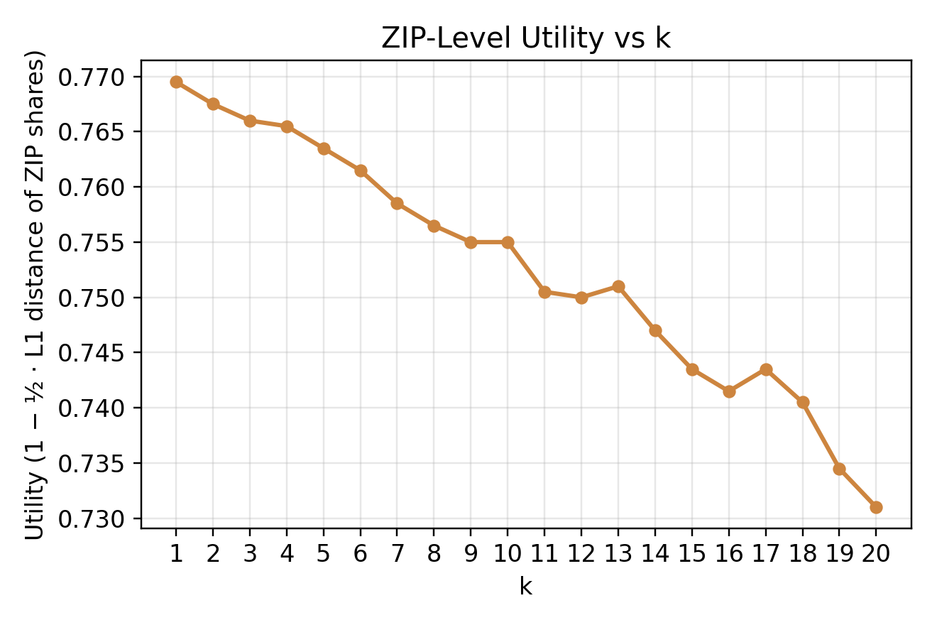
The line shows that as k increases, the ZIP code distribution retains less and less of its original detail.
Once k exceeds about 8, we see a notable drop in ZIP Utility.
At k = 16, roughly 25–30% of the geographic granularity is lost.*
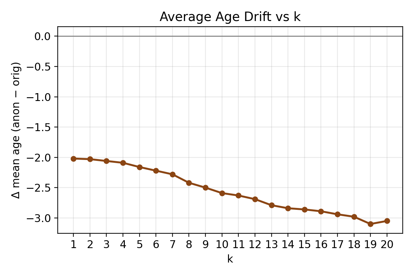
A negative drift means the anonymized data’s average age is lower than the original.
At high anonymity levels (k ≈ 20), the mean age is about 3 years lower.
Top-coding and heavy binning compress the age distribution toward the middle.*
Reassuringly, Mean Glucose remained essentially unchanged across all k values (drift ~0).
This confirms that the anonymization procedure targeted only QIs (age, zip, sex) and did not distort unrelated attributes.
Overall:
- For small increases in k (1–5), utility remains close to original fidelity.
- Beyond k ≈ 5–8, generalization becomes aggressive and utility drops sharply.
This suggests a “sweet spot” where privacy improves significantly while preserving substantial utility, after which additional privacy becomes expensive in terms of information loss.
The Privacy–Utility Frontier
It is helpful to visualize the inherent trade-off between privacy and utility.
Each anonymization configuration we tested
(a specific combination of k and generalization parameters)
can be thought of as a single point in a two-dimensional space:
- one axis = privacy outcome (e.g., Hit@1 re-identification success)
- the other axis = utility outcome (e.g., how many candidate matches remain / how much detail is preserved)
Plotting all configurations reveals a clear privacy–utility frontier.
Each point represents one anonymization scenario (specific k and parameter settings), plotted by its resulting privacy risk (y-axis: Hit@1 success rate) and a utility indicator (x-axis: number of plausible candidate matches per anonymized record, which correlates with retained information).

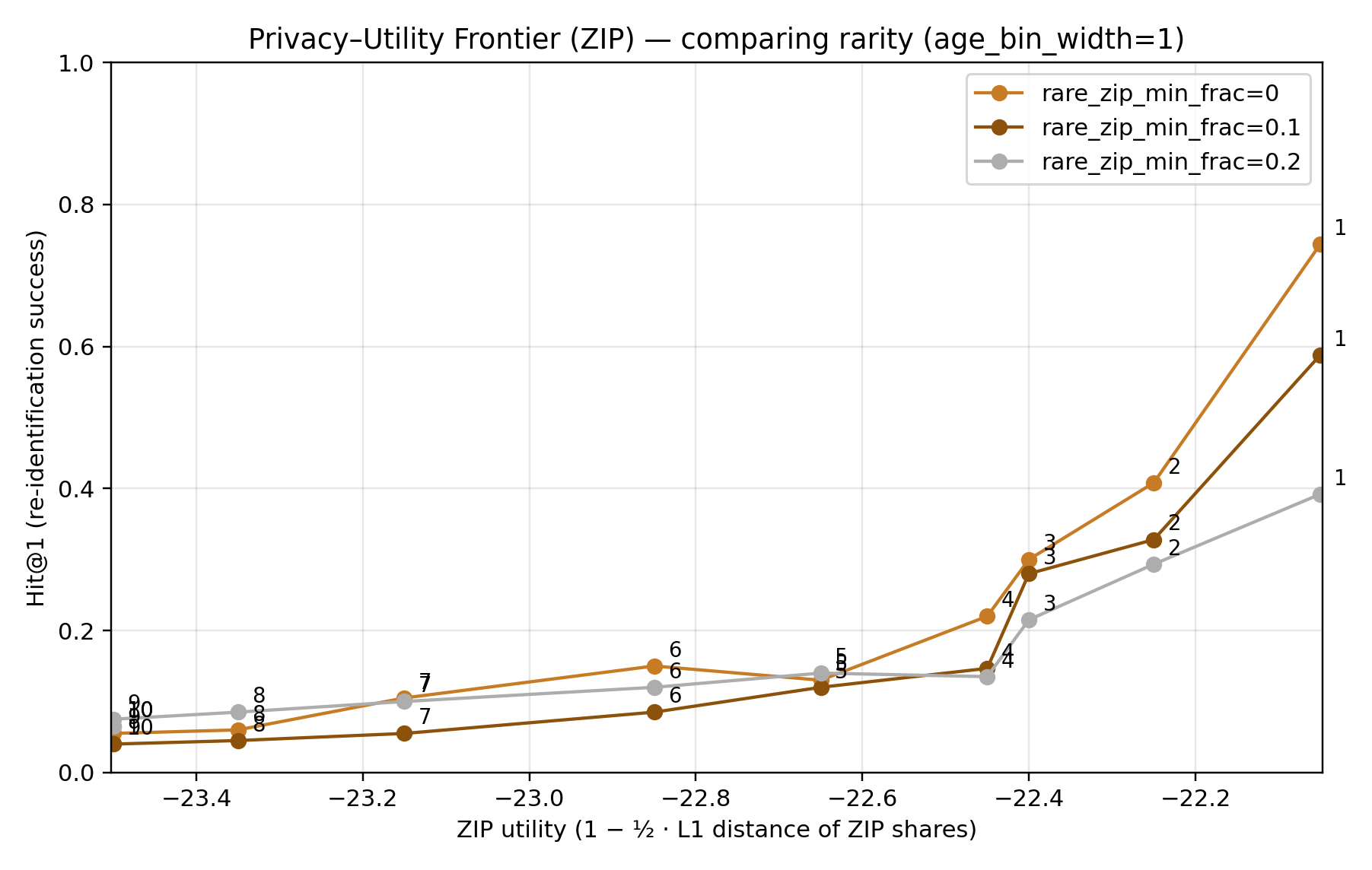
The plot forms a downward-sloping curve.
- Configurations with lower re-identification risk invariably have lower data utility.
- The initial part of the curve is steep — meaning you can reduce risk significantly with only a small drop in utility.
- The later part of the curve flattens — meaning achieving tiny extra privacy gains requires large utility sacrifices.
In simpler terms:
You can’t have it all.
Past a certain point, making the data “very anonymous” makes it statistically or analytically blurry.
The scatter shows every dataset version lies somewhere on this curve.
Deciding where to operate is a policy choice:
- low k → high utility, low privacy
- high k → high privacy, low utility
Conclusion and Discussion
Our empirical exploration highlights how increasing k-anonymity leads to diminishing returns.
For modest anonymity levels (up to around k = 5):
- Each increment in k yields a big drop in re-identification risk.
- The corresponding hit to data utility is mild.
Beyond that, however, the trade-off worsens:
- Pushing k higher gives smaller and smaller privacy benefits.
- Meanwhile, it rapidly erodes the granularity and usefulness of the data.
This is essentially a manifestation of a Pareto frontier —
there comes a point where you must give up a lot of utility to get a little more privacy.
Attribute Sensitivity
Different data attributes showed different sensitivity to anonymization:
-
Geographic detail (ZIP3) degraded first.
Many ZIPs are rare → must be collapsed to"Other"as k grows. -
Age was more resilient but eventually smoothed by
wide bins and top-coding → resulting in shifts such as
a 3-year drop in average age at high k. -
lab_glucose remained unchanged.
Since glucose was not part of the QIs, anonymization preserved it.
This demonstrates that non-identifying variables can remain intact
even as identifying information is stripped away.
This attribute-by-attribute difference shows that utility loss is domain-specific.
Some features lose meaning faster than others under anonymization.
About the Attacker Model
It is also worth noting that our attack model was relatively basic.
We assumed the attacker only knows:
- age
- sex
- region (ZIP3)
And they use a straightforward optimal matching algorithm.
A more determined adversary might:
- have additional clues (e.g., approximate health measurements)
- access multiple leaks
- use statistical models to narrow matches
- use Bayesian linkage, ML-based scoring, or constraint solvers
Such an attacker could defeat k-anonymity more often.
Therefore the Hit@1 rates in our experiment may be optimistic.
Real-world re-identification risk could be higher.
This highlights that anonymization should not be:
a one-time, set-and-forget protection mechanism.
You must consider evolving threat models
and possibly combine k-anonymity with other techniques:
- noise addition
- perturbation
- differential privacy
- synthetic data generation
- secure linkage systems
Finding the Balance
Ultimately, choosing an anonymization level is about balancing privacy risk against data usability.
Our experiment puts concrete numbers on that balance:
- The initial drop in re-id risk (as k rises from 1→5) is encouraging.
- It means we can significantly protect identities without immediately destroying utility.
- But the flattening of the curve at higher k reminds us that
aggressive anonymization yields minimal extra privacy at huge cost.
Decision-makers should consider what level of risk is acceptable
given the purpose of the data.
For many cases:
-
Moderate k (enough to prevent easy pinpointing of individuals)
is sufficient and maintains usefulness. -
High k may make the dataset practically unusable.
Key Takeaways
-
k-anonymity trades precision for privacy.
Generalization and suppression remove detail from QIs. -
Privacy gains are strong at first, then plateau.
Beyond mid-range k, utility collapses faster than privacy improves. -
Utility loss is nonlinear and varies by attribute.
Sparse attributes like ZIP lose meaning earlier. -
Non-identifying attributes can remain intact.
Good for preserving analytical value. -
Past moderate k, returns diminish greatly.
More anonymity → minimal privacy gain, major utility loss.
In conclusion:
Effective anonymization is about finding the balance:
protecting individuals without rendering data barren for analysis.
Our findings illustrate that balance clearly for this dataset under different settings.