
Code: github.com/mpcsb/tb-llm-distillation
An LLM can label a text-classification dataset without building a task-specific model first. It is useful, but the labels are not ground truth. Mixed evidence, vague language, and neighbouring classes can all produce inconsistent answers.
That leaves a more interesting question:
Once a student model has learned most of the task, where should the next unit of labelling budget go?
Probably not towards another random batch. Much of it will repeat what the model already knows. Instead, the student can help find weak class boundaries, questionable labels, and the kinds of examples missing from the dataset.
It is also cheap to run. The LLM does the expensive labelling; the student handles the large, repetitive passes over training and unlabelled data, locally and on CPU if needed.
Using the student to check the labels
The usual distillation flow is one-way:
LLM labels examples → student learns labels → student is deployed
But once the student exists, we can run it over the data that trained it:
student predictions → disagreements → inspect labels and weak regions
A disagreement can mean several things:
- the LLM label is wrong;
- the student is wrong;
- the example is genuinely hard;
- the dataset contains too few examples of that kind;
- the class definition is unclear at that boundary.
Any of these is worth knowing.
Asking the LLM again is one way to check a label. The student gives us a second opinion over the entire dataset in one pass.
A binary classification experiment
I set up a small example using 3000 Amazon appliance reviews. An LLM assigned one of two labels:
defect: a concrete failure in construction, operation, durability, or intended performance;no_defect: all else.
The distinction is semantic. A one-star review can describe incompatibility rather than a defect. A mostly positive review can still mention a concrete failure. The LLM received the product and review text plus the labelling rules, but not the star rating.
I kept 400 rows as a holdout and used 2600 for development. A microsoft/deberta-v3-base student, trained only on the title and review text, reached 0.9 accuracy and 0.89 macro F1. There was room to tune it further, but this was enough to explore the idea.
The budget has two phases
Before using the student to choose new data, I wanted to know when it became useful at all. I trained the same architecture on increasing amounts of teacher-labelled data and kept the 400-row holdout fixed.
| Teacher-labelled rows available | Holdout macro F1 | Behaviour |
|---|---|---|
| 100 | 0.416 | predicted only the majority class |
| 250 | 0.416 | predicted only the majority class |
| 500 | 0.810 | first useful student |
| 1000 | 0.841 | boundary begins to refine |
| 2600 | 0.882 | full public run |
Each run reserved 20% of the available rows for validation, so the model fitted 80, 200, 400, 800 and 2080 rows respectively.
The important jump is between 250 and 500 labels. Before that, the student predicts only the majority class and cannot guide anything. At 500 labels it starts exposing disagreements and weak regions.
That gives us a simple rule: sample broadly until the student is useful, then spend more of the labelling budget around its errors. These are single training runs, so the exact jumps will move around, but the two phases are clear enough.
I then ran the student over both the training and holdout sets, turning it back on the labels it had learned from.
The student disagreed with 65 of 2600 training labels and 39 of 400 holdout labels. I reviewed those 104 rows using the original prompt and changed 29 labels: 19 in training and 10 in the holdout set.
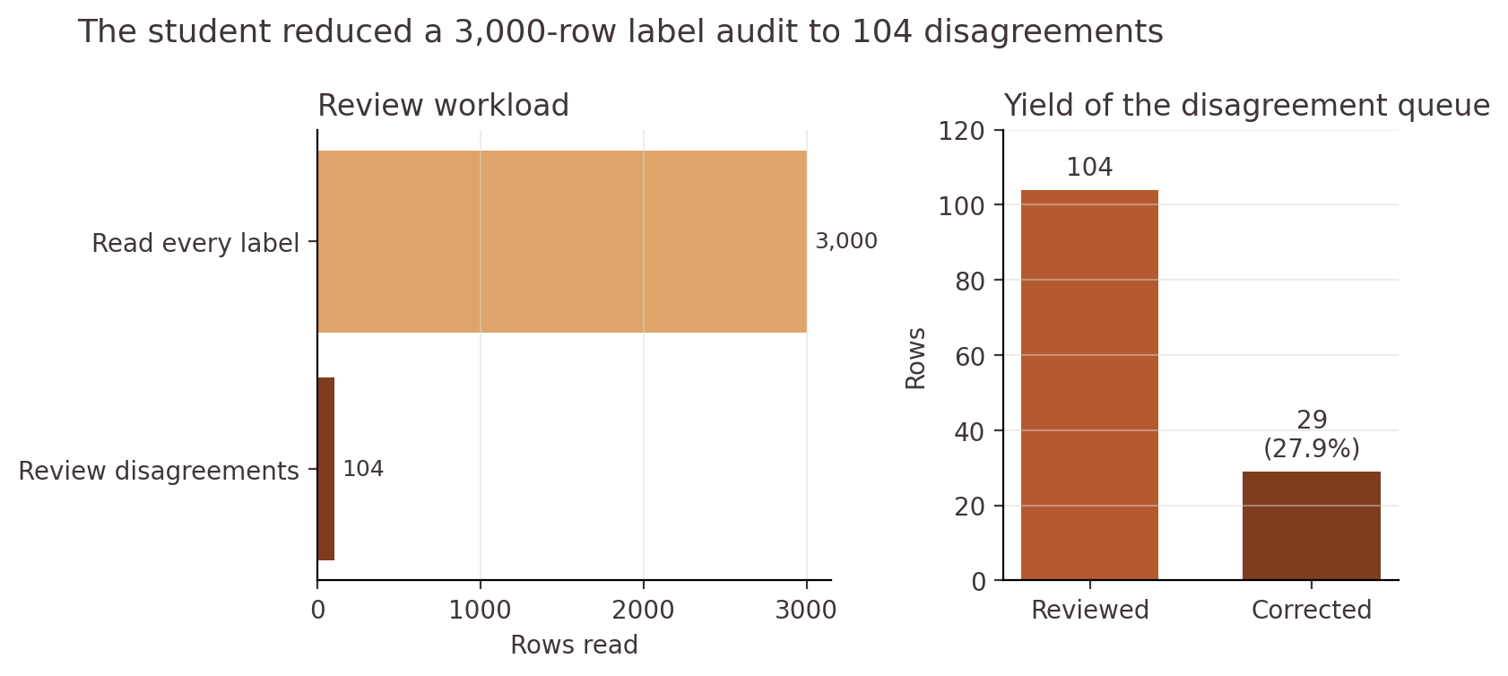
Reading 3.5% of the dataset found 29 labels worth correcting. More than a quarter of the reviewed disagreements were label errors.
The disagreements were not automatically correct. Some of the student’s most confident predictions were obvious model mistakes:
| Shortened review | LLM label | Student | Truth |
|---|---|---|---|
| “Handle attachment is chipped and sharp out of the box” | no_defect |
defect |
label wrong |
| “It didn’t seem to be filtering anything” | no_defect |
defect |
label wrong |
| “WAY too big to fit my regular stove” | no_defect |
defect |
model wrong |
| “Hinge came broken … holes had no threads” | defect |
no_defect |
model wrong |
The queue still needs review; it is not an automatic relabelling system.
Low-confidence sampling alone would miss much of this. Many useful disagreements were above 99% student confidence. Confidence tells us how strongly the student prefers one label, not whether the LLM label is correct.
Finding the next examples to label
Correcting labels is useful, but the student can also help choose what to label next.
I used this on a separate project with three ordered classes: A, B, and C. I cannot publish the domain or data, so the classes are anonymized and the results below are shown only in aggregate.
If most errors are A ↔ B and B ↔ C, we already know two things:
- which boundaries are weak;
- which parts of the class interiors do not need more budget.
We can then search an unlabelled pool for examples near those boundaries. Candidate-ranking signals include:
- the two largest class probabilities and their margin;
- disagreement between different models;
- nearest neighbours with mixed labels;
- keywords or phrases associated with known failures;
- source, category, time, or other metadata;
- repeated-group behaviour, such as several examples from the same source disagreeing in the same direction.
None of these should assign the label. They only help rank examples for the LLM or a human to review.
Even a crude keyword rule can help here. It may be a poor classifier over the whole dataset but a good retrieval mechanism for a rare, high-value slice.
What looks useful also changes after retraining. Once one boundary improves, another may become the problem. That is why I prefer small rounds with a quick student rescan between them, rather than one large batch based on the first model’s errors.
The task was difficult. No keyword or simple rule separated neighbouring classes, and many border cases were hard even for people to resolve consistently. A disagreement did not always mean the LLM was careless. Often the example was genuinely ambiguous and the dataset needed either better coverage or a clearer rule.
I ran the model over a large unlabelled pool, took the top two class probabilities for each row, and grouped the examples by boundary. After removing training rows and duplicates, I ranked the rest by probability margin and limited repeated sources. This left:
| Boundary | Candidates found | Selected for review |
|---|---|---|
A ↔ B |
~1400 | 500 |
B ↔ C |
~700 | 500 |
A ↔ C |
~250 | 250 |
The adjacent boundaries had far more unresolved examples than the outer A ↔ C boundary. That was useful by itself: it showed where the dataset needed work.
The selected examples were labelled and added in successive rounds. Additional queues came from confident disagreements on existing training rows and from weak keyword/metadata heuristics over the unlabelled pool.
With the architecture fixed at DeBERTa-v3-base and the same holdout throughout, macro F1 moved from roughly 0.862 to 0.870 over the data rounds.
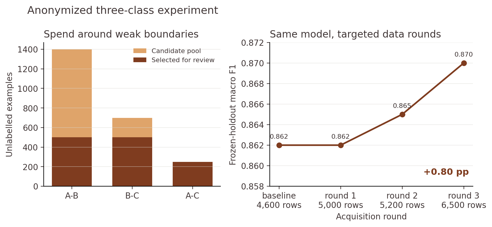
The rounds used different targeted sources, so this does not show that every targeted batch beats a random one. A proper comparison would put each batch against an equally sized random sample.
Still, the same model improved as I added data around its known weaknesses. In a separate correction round, changing only about 50 labels moved macro F1 by roughly two percentage points. Small edits can move a boundary when the rows sit in the right place.
Data is not the only lever. Once the labels are consistent and the weak regions have better coverage, persistent errors may point to model capacity. In this experiment, moving to a larger student on the same data added another 1.8 percentage points of macro F1. That is worth trying when the task depends on long context or subtle language, but not as the first response to a noisy dataset.
My order would be: fix the supervision, add data where it is missing, and increase model size only when the remaining errors suggest that the smaller student lacks the capacity for the task.
The complete loop
The loop looks like this:
1. Ask an LLM to label a broad, diverse seed set
2. Train a smaller student model
3. Run the student over training and validation data
4. Review confident teacher/student disagreements
5. Count errors by direction and identify weak class boundaries
6. Use uncertainty, neighbours, keywords, and metadata to rank unlabelled rows
7. Label a small targeted batch
8. Retrain and evaluate on a frozen holdout
9. Compare the targeted batch with an equal random batch
10. Repeat only where the marginal gain justifies another label
Keep three separate datasets:
- training data, which the model is allowed to shape and audit;
- acquisition data, from which the next candidates are selected;
- frozen evaluation data, which cannot be used to choose those candidates.
Otherwise it is very easy to improve the result simply by tuning against the test set.
Final remarks
LLM-labelled data should be treated as a first version of a dataset, not as ground truth. The student will also be wrong sometimes, so disagreements still need review. But once it becomes useful, it can point us towards bad labels, weak boundaries, and gaps in the training data.
Distillation leaves behind more than a smaller model. It also gives us a cheap way to question the dataset: bootstrap with the LLM, probe with the student, and spend the next label where it can still teach the model something.
Do not spend the labelling budget teaching the model what it already knows.