Why study model calibration under noisy data?
A few years ago, Claudia Perlich wrote on Quora:
“If the signal to noise ratio is high, trees tend to win. But, if you have very noisy problems and the best model has an AUC < 0.8, logistic beats the trees almost always. Ultimately not very surprising: if the signal is too weak, high variance models get lost in the weeds.”
That stuck with me because it contradicts the common instinct to reach for deeper or more powerful models when the data gets messy.
I wanted to revisit that claim, reproduce it in a small controlled setup, and then extend it a bit:
What happens when we add feature noise instead of switching labels?
And how does calibration (how well predicted probabilities align with reality) change under both types of noise?
TL;DR
- Logistic regression holds up well as noise increases, but it was already the best match for this dataset.
- Its smooth boundary is there by design. The interesting part is that its performance is not very sensitive to the noise added here.
- The tree models stay close on AUC, although the random forest has worse calibration.
- Calibration helps in places, mostly with the random forest. It is not a fix for lost signal.
Approach
The idea was to simulate a clean classification problem and then contaminate it in a controlled way.
- Data: 10 features, 5 informative, synthetic binary target generated with scikit-learn’s
make_classification. - Noise:
- Label noise: randomly flipping 0↔1 with probability p before the train/test split, so both training and evaluation labels are corrupted.
- Feature noise: adding Gaussian or Laplace perturbations, scaled to each feature’s standard deviation, before splitting the noisy data into training and test sets.
- Models:
A logistic-regression pipeline with pairwise interaction features, random forest, and XGBoost, with and without isotonic calibration. - Metrics:
AUC for discrimination; Expected Calibration Error (ECE) for reliability.
The run uses 3000 samples and one split per noise level. It is a small experiment, not a definitive comparison of model families.
Results
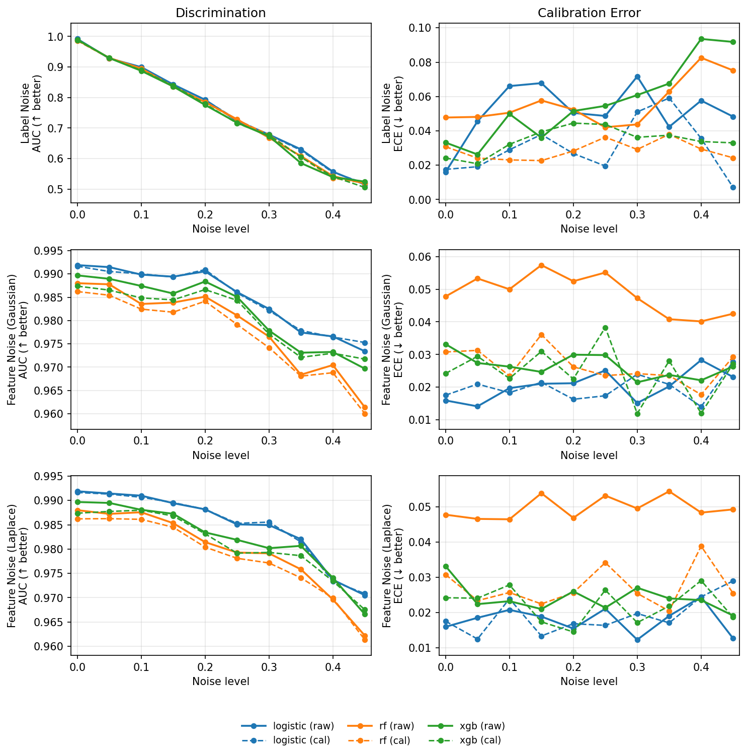
This is what I see in the plot:
- Under label noise, all models decay almost in lock-step. Labels are flipped before the train/test split, so the test labels are noisy too. As the flip rate approaches 50%, the labels stop meaning much and AUC moves towards 0.5.
- Under feature noise:
- AUC drops only a little for all three models. Logistic is slightly ahead for most of the tested range.
- The raw random forest has the highest calibration error.
- Isotonic calibration (the dashd lines) usually helps the random forest. For logistic regression and XGBoost, it is less consistent.
What does “stable” mean here?
The smooth curves need a bit of care. Logistic regression gives us a smooth score surface anyway; that is just how the model works. It does not mean the model is somehow reacting smoothly to noise. What the plot shows is simpler: its AUC doesn’t really move as feature noise increases. In this setup, it is robust to noise.
Why does logistic perform well here? Mostly because the problem suits it. It already has the highest AUC before any noise is added. make_classification gives us a fairly simple synthetic structure, and the pipeline adds pairwise interactions before fitting logistic regression. So it is not even strictly linear in the original features.
Adding noise did not create its advantage; it was ahead from the start.
This matters because real data is not always shaped like this. It can have thresholds, interactions, and cycles such as hour of day, day of week, etc. Sometimes a few extra features, like sine/cosine or fourier decomposition, are enough. Sometimes a nonlinear model is simply a better fit.
So I would not take this as proof that linear models are generally more stable than trees. It shows that a relatively simple model can be hard to beat when the problem already suits it.
Conclusion
The logistic pipeline loses very little AUC under the feature noise tested here. That fits Perlich’s observation, but there is a simple reason for it: the model already suits the generated data.
Calibration helps the random forest probabilities, but it cannot bring back signal that is gone. The practical takeaway is to start simple and test with noise that looks like the real problem. A basic model can be hard to beat when its assumptions fit the data. When they do not, simplicity will not save it.
Check the code and adjust noise distributions, switch datasets, try out different models. Have fun!