This is the continuation to this post where we explore the changes in the output of machine learning models when they are trained on samples of varying sizes.
Some preliminary thoughts and conclusions from the last post:
- Complexity of the models determine how profitable it is to explore in lower samples. For quadratic algorithms and ignoring the actual implementation, training one model with a full dataset should cost the same amount of time as training 6.25 with 40% of that dataset.
- Before a threshold sampling percentage, the results of a model are not informative for the full dataset. Being greedy doesn’t help here.
- Overall, models at smaller samples seem to be noisier images of the full dataset trained models.
Let’s take this example from bayes_opt.
We want to optimize over a 3d space composed of random forest parameters (max_features, min_sample_split, trees) where the model is evaluated a cross-validated negative log-loss score.
A standard bayesian optimizer runs 100 models with a synthetically generated dataset with a binary target.
Let’s do a run in an exploratory mode: focusing one exploring the landscape instead of necessarily exploiting regions near local or global maxima.
The logs below print how many models were ran during the bayesian optimization and the computational budget it consumed.
We print the best combination of parameters until the last iteration. During this process, the best model was found in iteration 13 and the remaining 87 never resulted in a superior model.
Optimizing Random Forest: 100 models; budget: 100
|   iter    |  target   | max_fe... | min_sa... | n_esti... |
=============================================================
|  4        | -0.3418   |  0.4902   |  0.02077  |  10.02    |
|  8        | -0.3349   |  0.6166   |  0.01651  |  10.02    |
|  13       | -0.2919   |  0.999    |  0.01     |  250.0    |
=============================================================
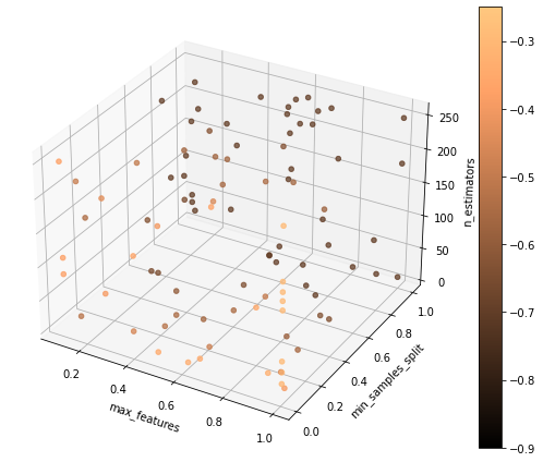
The figure below shows a fairly explored space, where some regions clearly seem to have more performant models (lighter tone in the color scale).
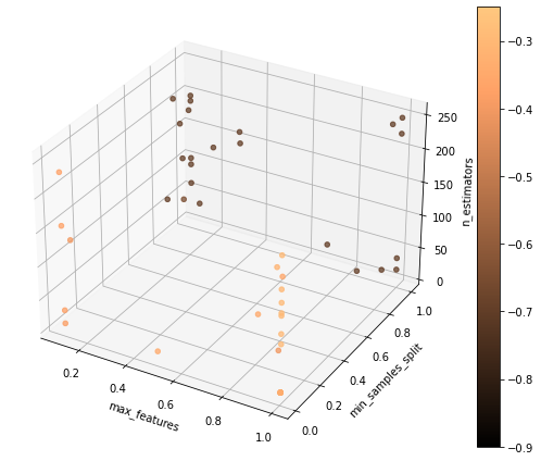
Another run promoting a more balanced relation between exploration and exploitation:
Optimizing Random Forest: 100 models; budget: 100
|   iter    |  target   | max_fe... | min_sa... | n_esti... |
=============================================================
|  4        | -0.3423   |  0.4902   |  0.02077  |  10.02    |
|  5        | -0.3404   |  0.999    |  0.01     |  10.0     |
|  6        | -0.3149   |  0.9771   |  0.01587  |  188.5    |
|  12       | -0.2959   |  0.999    |  0.01     |  96.31    |
|  16       | -0.2946   |  0.999    |  0.01     |  141.4    |
|  51       | -0.2943   |  0.999    |  0.01     |  122.7    |
|  95       | -0.2942   |  0.999    |  0.01     |  126.5    |
=============================================================
Both strategies seem to be effective exploring the parameters. Let’s add subsampling to it.
To benchmark all the variants in the exploration we fix the same compute budget, that is, the same that is needed to run 100 models with the full dataset.
Let’s consider negligeble the compute time for the gaussian process that fits the hyperparameter space, even though it isn’t: 1) as observations grow; 2) as the hyperparameter space grows; 3) and if the model function is not too expensive to compute.
Some remarks:
- The computational budget is divided between different sample sizes, and for each size, we can quantify a quantity of models given by the complexity relation. Random forests are assumed to be log-linear; SVMs are considered to be quadratic. Abstracting some implmentation details is acceptable to get started.
- The lowest percentage which samples the dataset is fixed and it should be tuned depending on the complexity of the data. 1% of the data may be enough to learn the target.
- How many sample sizes should we explore? Not enough has been explored here, but it seems to be again contingent on the data.
- What strategy to use when dividing the budget: evenly over the various sample sizes or something more complex?
The key concern once the exploration in a sample is completed, is how to pass the information gathered and pass it to the next (larger) sample exploration.
A simple step is to pass promissing points to probe; adjusting the domain of the parameters in order not to explore flat areas is promissing but not easy to implement in bayes_opt; another simple way to pass information is to copy the posterior (after fitting to the observations) covariance function of the underlying gaussian process and use it as a prior to the optimization process of the following sample.
Some ideas to make subsampled bayesian optimization more clever where: 1) to make the strategy of exploration sample size dependent. Exploring at lower samples and exploiting at higher samples seems a good heuristic; 2) to add a noise term to the gaussian process that is dependent on the sample size. This is to model the higher variance at lower samples.
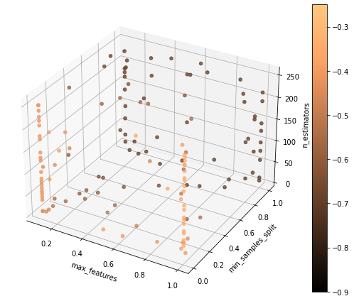
The logs and figures below show the result of a 3 sample size split, with sample percentages in the following set: [30%, 70%, 100%], where the computational budget (the equivalent of training 100 models with the full dataset) was split evenly.
Notice that the same budget allows for a very different amount of models at each sample size. Allocating more budget to lower or higher percentages could ease the exploration of more complex parameter spaces.
Sample percentage:30%
Optimizing Random Forest: 148 models; budget: 33
|   iter    |  target   | max_fe... | min_sa... | n_esti... |
=============================================================
|  4        | -0.3858   |  0.4902   |  0.02077  |  10.02    |
|  9        | -0.3753   |  0.9791   |  0.01979  |  23.29    |
|  19       | -0.3539   |  0.6998   |  0.02344  |  241.5    |
|  43       | -0.3354   |  0.999    |  0.01     |  221.5    |
|  112      | -0.3344   |  0.999    |  0.01     |  46.79    |
|  137      | -0.3343   |  0.999    |  0.01     |  40.97    |
=============================================================
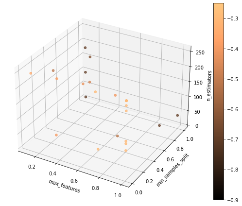
Sample percentage:70%
Optimizing Random Forest: 57 models; budget: 33
|   iter    |  target   | max_fe... | min_sa... | n_esti... |
=============================================================
|  3        | -0.3023   |  0.999    |  0.01     |  114.4    |
|  5        | -0.302    |  0.999    |  0.01     |  234.8    |
|  42       | -0.3006   |  0.7511   |  0.0109   |  67.98    |
=============================================================

Sample percentage:100%
Optimizing Random Forest: 33 models; budget: 33
|   iter    |  target   | max_fe... | min_sa... | n_esti... |
=============================================================
|  32       | -0.2917   |  0.7301   |  0.01     |  250.0    |
=============================================================
To conclude, this was not an exhaustive search of how subsampling can be used to search optimal points in the hyperparameter space.
The code below can be changed to:
- Explore different budget dividing strategies;
- Explore different amounts of noise in each of the sample percentages;
- Investigate how to leverage the exploit vs explore trade-off;
- Explore some relation between the observed points and the number of points to pass across samples;
- Explore how different these points should be;
…
The exploration of higher dimensional spaces at lower samples seems at least more effective than relying on very expensive model full dataset training. For models with higher complexity this should be evident.