Modeling time series outliers with Gaussian Processes
This is essentially a back of the envelope study for the identification of outliers in time series. The idea is to sketch a method that associates model quality to the presence of outliers.
When dealing with data which does not follow time, finding outliers is hard, but even simple approaches might yield decent results. Setting a threshold for the percentile that determines what is a classifier works nicely in one dimensional data, and might even be useful in low dimensional data. To make sure, add a Bonferroni Outlier test and whatever you decide, it has some support.
For time series that evidently not a satisfying answer. Even very rare values can be periodical; this is in fact a common pattern.
One definition of outlier is a measurement that does not fit with the data generating process.
For a sufficient amount of samples, the signal makes itself clear, even when in presence of significant noise. Let’s focus on the problem with a small amount of data points — something like monthly series, a frequent business scenario.
Let’s create a small series which has the following decomposition:
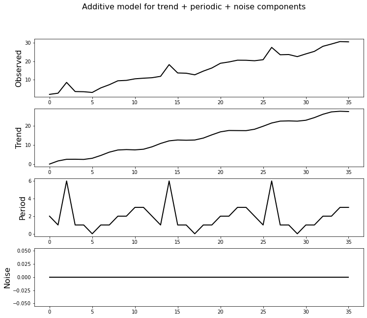
We need to create a generating model which will be critical to evaluate the likelihood of a point being an outlier. Let’s not use the entirity of our knowledge of the series.
For a series this simple, we’ll use a gaussian processes regression, and we’ll define the covariance function as the sum of the Matérn 5/2 kernel and a periodic kernel of period 12. We also define a linear mean funcion, with the slope defined with by a random variable that is inferred using MCMC.
This is as a plausible injection of basic yet informative priors to the model. More complex series may require complex models, which are harder to sample and harder to illustrate the idea of the post.
A quick test, performing a 12 month forecast, shows the model capturing the signal pretty well when there is no noise, and as the noise magnitude increases,the predictive ability decreases, as expected.
One particular feature that I enjoy in gaussian processes is the ability to interpolate data very nicely and allowing imputation of missing values in a principled way. Because we can draw samples from the model, we can generate distributions for each of the points in the series. We exclude each point and, assuming the model is sufficiently well defined, we could collect percentile values for the values of the series.
Now, the outcome of this step seems redundant or a symptom of a weak model/a hard problem to model. However, the main objective is to show that the absence of outliers will generate a superior model, that reduces the modelling error significantly for the rest of the series.
This extra iteration over the entire series adds a significant amount of computing time to an already complex method — but this is a small series and a few seconds per model is nothing obscene Below we get to see the process for the series with minimal amount of noise.
Even with a model that’s as close to naive as possible, the signal is picked and for the most part the mean of the samples matches the missing value.
The key idea behind this post is the superior model that is trained when outliers are removed from the time series. This is something made clear in the next animation. When the outlier is removed, the variance of the model is very low compared to the models generated when it’s not, and most importantly, the mean of the samples of the posterior resembles the original time series.
In case of more than one outlier, the problem stops being trivial; the absence of one of the outlier is no longer sufficient for the model to obtain a clear signal — depending on the magnitude of the outlier, the perturbation it adds makes any modelling quite hard, forcing the removal of another data point.
We can see the model seems to improve when any of the outliers are removed; measuring this improvement might be sufficient to list outlier candidates and then removing the combinations of elements of this list to find out the most promising set.
It’s still hard to generate some heuristic that generalizes for most outliers — any value with an offset large enough from the original time series is easily detectable, but after removed, requires one additional loop over the remaining points; even with a small amount of data, it gets prohibitive.
The main conclusions taken from this post is that outliers are hard to evaluate, unless if specific cases.
Here, knowledge of the system was needed to build a good enough model; of the amount of noise that influences the process ; and the of how many outliers are in series were essential. In a real world scenario, this is not the case, but it may still serve as an exploratory step.