This is the first of two posts about finding optimal parameters for machine learning models, and is motivated by Hyper-Parameter Optimization: A Review of Algorithms and Applications. Subsampling is commented on a later section, as a strategy to reduce the training time; and doing so, reduces the search time for necessary to find optimal values. It’s stated that subsampling is risky in terms of the potential to introduce more noise and uncertainty.
On this first post I’m going to explore subsampling and how much can be learned about the parameter space from it. Try to find support from observations that the parameters tend to converge to the some value as training data increases, and if it seems to increase at the same rate for all parameters; observe the effect in combinations of parameters; and to see if the overall patterns generalizes in the same way to different methods.
On the second post I’ll use subsampling to explore the parameter space, using whatever computational budget there is, efficiently.
Predictive models are able to generalize what they learn from data, otherwise they’re not very useful – but there is a minimum amount of data which serves as a boundary for the lack of learning ability of the model.
Let’s pick then the Random Forest implementation by sklearn, and pick three parameters as a start. The data is the Boston housing dataset, around 500 records which is a nice amount to perform some grid searches for these initial tests. I’ll track the R² score obtained from cross validation.
What we expect to find is evidence that smaller samples are still informative to find the optimal parameters of the full dataset.
For each size and combination of parameters, we randomly sample from the original dataset, while keeping the random seed of the algorithm to maintain some amount of determinism.
The plots below show the results for grid search for the parameters. Keep the colorscale in mind; it’s used for the rest of the plots.
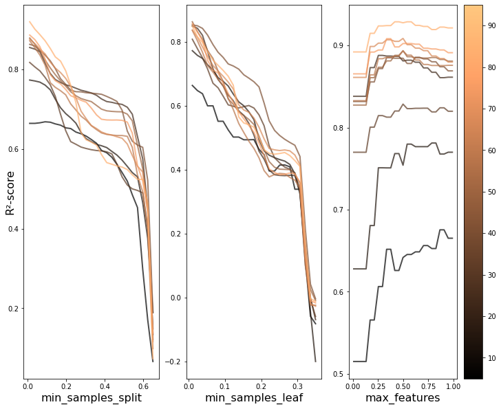
Some comments:
- Less data means less to learn: the performance must necessarily be smaller with small samples.
- Less data means greater variation in how the training data can be generated – some combinations can be very unrepresentative of the dataset. This needs to be explored further.
- For some parameters – max features – subsampling seems to have a greater impact on the predictive performance of the model.
As expected, the parameter curves seems to share a lot of features across sample sizes, even at the smallest ones, and as the size increases the convergence seems to be even more apparent. To put it simply, the optimal parameters are quite similar after a certain size.
Let’s explore the variation of the scores a bit further.
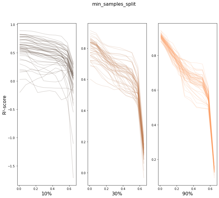
Let’s focus on one parameter, min_sample_split and repeat the exploration a few times.
And we can see the mean value and the region of the two standard deviations.
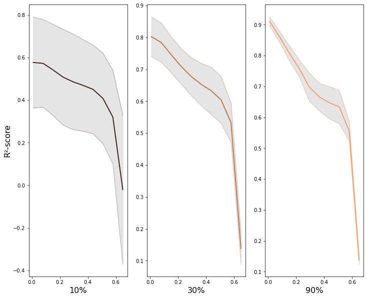
Smaller samples have a greater variance than larger samples – there are certainly odd combinations, in particular for a small dataset as this one.
Larger samples will have a significant overlap with the orignal dataset which means that there’s less to vary in the training data, and as expected, the results are much less scattered.
In my implementation, even when the sample sizes matches the entire dataset, the order is not fixed by a random seed and is not kept; this adds additional variation, which is not only acceptable, but actually desirable to explore the what causes different outcomes in these methods, and to get an idea of the magnitude of the variation.
Before trying to observe the same patterns hold in other scenarios, let’s take a minute and explore, fixing one parameter, the distributions for the scores at each sample size. The reason is to start observing the actual dynamics of these distributions as more data gets fed to the model.
Below we can see that if we exclude very low sample sizes – there is a very significant overlap in the R² scores distributions. In other words, there is plenty of useful information at lower samples.
On interesting aspect of these repeated draws at a specific sample size seems to be the bell shape of the distribution. Even with ceiling effects, normality tests are passed and we can at least use this as information to model the behavior in the second post.
One continuation to this exploration needs to be related with the relation between sample size and more than one parameter.
We have two examples of combinations of parameters that support what we saw previously: the surfaces share plenty of similarities for various sample sizes, and most importantly, the parameters that maximize the R² score seem to be at the very least neighbours and at the very best the exact same.
One comment regarding how different datasets affect what we have observed. There seems to be a point in the sample size after which the dataset is informative enough for the model to pick up patterns. Rich datasets are a bit more demanding when it comes to how small samples can be – this adds another layer of variance to what we see and that is ignored for now.
One final exploration with a SVM is carried out. There is no scaling of the features or anything remotely trying to maximize the performance; again, the point is to see that there is no dramatic changes to the model behaviour.
We can see that for the very smallest sample size, the maximum seems to be contested by two distinct locations in the parameter space. Small samples are troublesome as we’ve seen and different algorithms scale differently.
The second smallest sample already seems to converge to the optimal set of parameters and at this point we can make some comments that motivate the next post.
Our first method was the random forest, which scales nicely, log-linearly. SVMs on another hand have quadratic time complexity, and this is one aspect to explore and that motivates subsampling in this exploration.
To compute one model with the entire dataset it costs us the same as the cost of training seven in the second smallest sample size: there is intrinsic noise that comes from small samples, yet we can explore a lot more.
A structured, yet simple, approach to how this exploration can be made, leveraging the trade-off between information gained and reduced computational load, is the content of the next post.