This note walks through a simple but realistic case where Bayesian logistic regression helps simulate pricing scenarios — a model based way to explore sales decisions.
Why use Bayesian regression for model based simulations?
In this post, we’ll build a simple probabilistic model and use it to simulate a few scenarios.
Linear models handle noisy observations well — they stay focused on the main signal instead of chasing small fluctuations. Bayesian regression adds key advantages: we can encode domain knowledge as priors, quantify uncertainty directly from the posterior, and express results as probabilities rather than p-values or arbitrary confidence intervals.
For exploring counterfactual or simulated scenarios, that mix of simplicity and principled uncertainty is exactly what we need.
Case Study
A good example for this kind of modeling is converting sales opportunities.
Sales reps typically log opportunities under their accounts, along with details such as the offered unit price and whether the deal was ultimately won or lost.
Some of these attributes are naturally informative, and, as with most purchases, price is often the dominant factor behind the conversion.
Still, the data doesn’t capture everything. Competitor pricing, credit limits, or internal approval rules can all affect the outcome, and their absence adds noise to the target variable.
Because we understand this process and the role of price so well, it makes an ideal test case for a simple Bayesian model.
Data
We’ll start with a small simulated dataset of 500 sales opportunities.
Each record has a conversion status (won = 1, lost = 0) that depends mainly on the unit price offered, along with two categorical attributes — the account country and the product ID.
Each product and country has its own coefficient, representing factors such as sales-rep behavior, discounts, or product-specific promotions.
(A full hierarchical version could share information across groups through hyperpriors, but here each level is modeled independently for simplicity.)
Additional random variation is included to capture unobserved factors that influence conversion — for instance, market competitiveness or credit conditions.
A sample of the dataset is shown below.
For simplicity, the model will ignore the amount column (informative but unnecessary here) and focus on unit_price, country, and product ID.
| id | unit_price | p_id | amount | country | status |
|---|---|---|---|---|---|
| 325 | 30.342365 | 4 | 62.734691 | a | 1 |
| 457 | 69.475791 | 5 | 20.922939 | c | 0 |
| 351 | 30.164137 | 4 | 73.612906 | b | 1 |
| 224 | 2.851734 | 1 | 207.205554 | c | 1 |
| 123 | 39.875412 | 4 | 7.842334 | b | 0 |
Check the data generating code for the specifics.
The plots below show how the conversion target varies across the five simulated products and three countries.
The division follows the ratio of offered price to base price, though it’s not a strict boundary.
Higher simulation noise makes that division fuzzier and the classification problem harder overall.

Model
Let’s set up a simple model to study opportunity conversion.
This isn’t meant to perfectly fit the data — just a basic object for controlled simulations.
We’ll use PyMC3(now PyMC) to implement a Bayesian version of logistic regression.
If any part of the definition feels unclear, check their examples and docs.
The unit price values are normalized by each product’s base price.
This scaling keeps features near zero, which simplifies the choice of priors.
The model includes linear terms for product and country, along with a common intercept, and uses a logit link to map the linear predictor to probabilities.
These probabilities then define a Bernoulli likelihood for the conversion outcome.
Because we know price has the strongest influence, we’ll assign a prior that allows its coefficient to take relatively large (in magnitude) values.
Formally:
yᵢ = β₀ + β_prod[prodᵢ] + β_ctry[countryᵢ] + α_prod[prodᵢ]·priceᵢ + α_ctry[countryᵢ]·priceᵢ
pᵢ = sigmoid(yᵢ)
statusᵢ ∼ Bernoulli(pᵢ)
N=len(train_status)
dim1 = len(set(product_id))
dim2 = len(set(country))
with pm.Model() as shared_data_model:
intercept = pm.Normal('intercept', mu=0, sd=1)
alpha_product = pm.Normal('alpha_product', mu=0, sd=1, shape=dim1)
alpha_country = pm.Normal('alpha_country', mu=0, sd=1, shape=dim2)
sigma_beta = 10
beta_product = pm.Normal('beta_product', mu=0, sd=sigma_beta, shape=dim1)
beta_country = pm.Normal('beta_country', mu=0, sd=sigma_beta, shape=dim2)
train_cty = pm.Data("train_cty", train_country)
train_p = pm.Data("train_p", train_product_id)
train_offers = pm.Data("train_offers", train_normalized_offers)
train_p_cty = pm.Data("train_p_cty", train_p_cty)
p = invlogit(intercept
+ alpha_product[train_p]
+ alpha_country[train_cty]
+ beta_product[train_p] * train_offers
+ beta_country[train_cty] * train_offers
)
y = pm.Bernoulli('y', p=p, observed=train_status)
trace = pm.sample(init='advi+adapt_diag', n_init=100000,
tune=1000, draws=1500, chains=3, cores=8,
target_accept=0.90, max_treedepth=10)
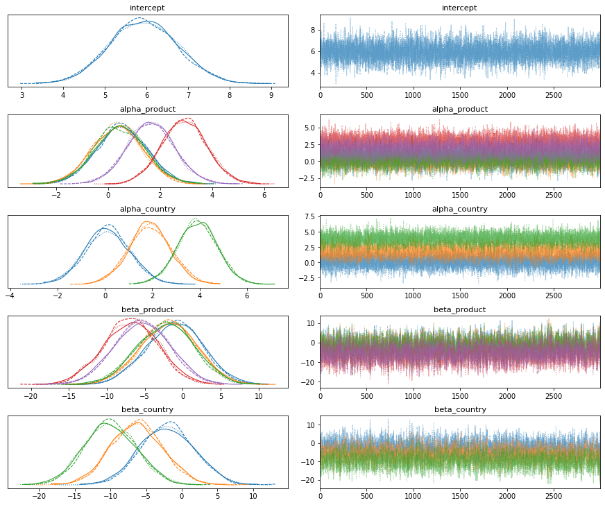
az.plot_trace(trace, compact=True); plt.show()
This model is simple enough for this dataset, so there are no divergences or other diagnostics raising concerns.
Let’s proceed.
For simple models like this, even weaker priors would likely be informative enough. Adding extra terms, for example, industry or time components, would increase complexity and make sampling harder.
When the data are noisy and the signal is faint, encoding knowledge through priors can help the sampler converge and stabilize inference.
Sampling from the posterior, we see that price cleanly separates converted from lost opportunities.
The highest posterior density regions show how conversion probability shifts with normalized price.
Alternative transformations, such as z-scoring price by product, produced slightly cleaner regions, but since model performance was identical, keeping the price as-is was more convenient for the simulations — the main focus of this post.
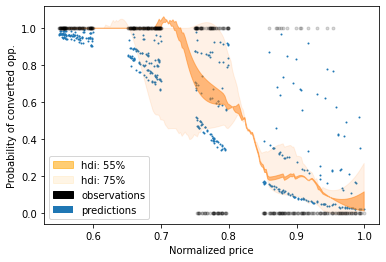
The key takeaway from this model is that when predicted probabilities align well with observed outcomes, the model’s predictive performance is strong.
Below we can see predictions on a hold-out set and the uncertainty of each, expressed as the standard deviation of their posterior predictive distributions.
This helps gauge how much trust to place in each individual prediction.
For a Bernoulli variable, the posterior standard deviation is bounded by 0.5 — uncertainty is highest near p = 0.5 and decreases as probabilities approach 0 or 1.

In addition to the posterior prediction spread, we can also assess model uncertainty by inspecting the posterior distributions of its parameters.
Parameters with wider posterior curves imply higher uncertainty, which naturally propagates into predictions.
Listing their standard deviations is an intuitive way to see why some predictions carry more uncertainty than others.
Simulations — Discounts and Mark-ups
Linear models extrapolate reasonably well, though they assume a linear relation.
That’s not always realistic — non-linear behavior appears when prices approach zero or climb far above the base level.
To explore what discount might turn a declined offer into a win, we can sample from the posterior at different price values.
The plot below shows how conversions evolve with discounts; color encodes uncertainty (posterior standard deviation) across previously lost opportunities.
Lower prices increase conversion probability, but products or countries with weaker signal-to-noise remain more uncertain.
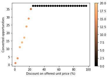
From the simulations, a discount of roughly 20% is enough to recover nearly all lost opportunities — beyond that, additional cuts bring little gain and simply erode margin.
The same approach applies to price increases: we can examine how higher unit prices trade off revenue versus conversion loss.
The figure below shows the decline in wins as prices rise — useful for identifying thresholds just below where business begins to drop.
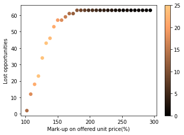
Both simulations behave as expected: lower prices drive conversions, higher ones reduce them, confirming the model’s internal consistency and our intuition about the problem.
This post hopefully helped illustrate how we can use models to assist in simulating scenarios.
More complex models will bring very interesting simulations, and optimizing these parameter landscapes will become a less trivial exercise.
Check the code and adjust noise parameters to explore different scenarios